Present and future of graph processing with Spark


Graphs have been around quite a while. In fact, the first paper in the history of graph theory was written by Euler himself in 1736! However, it wasn't until 142 years later when the term graph was introduced in a paper published in Nature. Despite those shiny names, graph applications remained fairly marginal until the development of computers, which made its use affordable for physical, biological, and social processes.
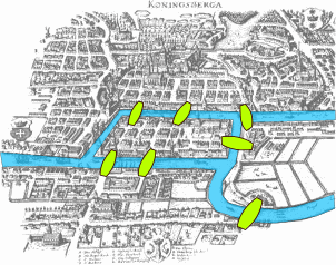
Euler tried to solve the Seven Bridges of Köninsberg problem that consists on devising a walk through the city that would cross each of the bridges once and only once. He proved it had no solution. Image By Bogdan Giuşcă - Public domain (PD), based on the image, CC BY-SA 3.0, Link
\[
\Biggl \lbrace \begin{array}{lr}
\frac{D\pmb u}{D t} = -\Delta w+\pmb g \\
\Delta \cdot \pmb u = 0
\end{array}
\]
Euler equations for adiabatic and inviscid flow (fluid dynamics).
Returning to the present, most internet companies use graphs as a core part of their business implementing Knowledge Graphs. Facebook, Google, Twitter, Netflix or Uber are some examples. Those graphs, usually with the RDF data model, are designed for fast online queries and used by a multitude of users, usually performing small queries with just a few levels in depth.
On the other hand, those companies also need powerful graph-crunching systems, more like Hadoop approach rather than MySQL. The most notorious example of this is Google, that developed the page rank algorithm which provided the most accurate results that ever existed at that time iterating multiple times over all the websites it indexed and its links. Another example is Facebook. They use and develop Apache Giraph, an open source implementation of Pregel algorithm using Hadoop's MapReduce. In fact, they scaled Giraph at least up to a billion (\(10^{12}\), trillion in the US) edges. This was in 2013, and I'm sure it has exceeded far beyond that point.
However, at this point I should warn you: the number of edges and nodes is not always a good quantifier. You have to keep in mind that usually vertices and relationships have properties. At least with enterprise graphs: the amount of a money transfer, the date of a new friendship, when and by whom a road was built, a user's birthday ... The amount of this kind of metadata depends on a broad range of factors, but two of them stick out: what do you pretend to do with the graph and the data modeling you have to adapt to. Most of the times when you implement a graph system to a company they ask you to build the graph with their data model, commonly inherited from a relational database, where tables with more than 100 columns are the standard. And I can assure you they will want to use a bunch of them.
These two aspects are important. It is not the same a graph with 3M nodes and 10M edges with no properties or the same graph with 100s of properties. The first has a size just under 300MB while in order to process the latter, you will probably need a badass server with 44 cores and 500GB of RAM. And besides the size, the functionality is a lot different! With a graph with almost no properties you can certainly run graph algorithms like shortest path, PageRank, connected components... but you won't be able to perform a wide analysis in order to detect complex fraud with subtle clues. To do so you'll need enriched data with metadata, geolocation, machine learning enhancements...
Anyway, I feel like I have rambled enough. Let's talk about the topic.
Spark and graphs, a love story?
Damn, I was lying: I must digress a bit more because in order to explain the difference between the two ways to work with graphs in Spark I need you to understand two different data structures. If you already know de difference please, skip the following section.
RDDs vs. Dataframes
Dataset[Row]).
Let's start with some definitions taken from Spark API and Spark Documentation:
A Resilient Distributed Dataset (RDD) is the basic abstraction in Spark. It represents an immutable, partitioned collection of elements that can be operated on in parallel.
Internally, each RDD is characterized by five main properties:
- A list of partitions
- A function for computing each split
- A list of dependencies on other RDDs
- Optionally, a Partitioner for key-value RDDs (e.g. to say that the RDD is hash-partitioned)
- Optionally, a list of preferred locations to compute each split on (e.g. block locations for an HDFS file)
A DataFrame is a Dataset organized into named columns. It is conceptually equivalent to a table in a relational database or a data frame in R/Python, but with richer optimizations under the hood. It is specially designed for SQL querying of distributed tables.
To sum it all, RDDs have a very low-level API, where optimizations depend on you, while DataFrames leverage the high-level SQL syntax to implement an optimizer between your code and the actual execution plan (see examples and explanation here).
In order to clarify, let me show you a toy example about the importance of operation order in both APIs: we have some CSV files that represent a table. We have two columns: city and population. We want to obtain the number of young people in Barcelona, knowing that approximately 20% of the population is under 25. We have at least two options: compute the number of young people per city in the entire data and then filter by city, or vice versa: filter first and then apply the computation.
If we use spark RDDs, the first option will cost double than the latter. First, you will compute a division for each entry in the data and filter later. However, if you filter first, then spark will only have to do one operation in the second step! Much more efficient.
On the other hand, the spark DataFrame (and Dataset) optimizer doesn't care about the order you wrote those operations. It analyzes all the process and it sees that you want to perform both operations, and internally it establishes the second option as a winner.
So, the main difference is in the level of abstraction and the optimizer.
Test data and objective
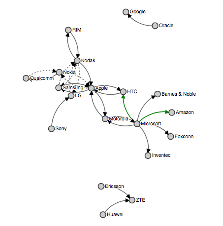
In both cases, we will use the following dataset so we can compare directly the usability. This toy data is taken from an example of the library D3.js and is comprised of the mobile patent suits between companies.
The following code is used to load the data into a DataFrame:
val raw = """{"source": "Microsoft", "target": "Amazon", "type": "licensing"}
  {"source": "Microsoft", "target": "HTC", "type": "licensing"}
  {"source": "Samsung", "target": "Apple", "type": "suit"}
  {"source": "Motorola", "target": "Apple", "type": "suit"}
  {"source": "Nokia", "target": "Apple", "type": "resolved"}
  {"source": "HTC", "target": "Apple", "type": "suit"}
  {"source": "Kodak", "target": "Apple", "type": "suit"}
  {"source": "Microsoft", "target": "Barnes & Noble", "type": "suit"}
  {"source": "Microsoft", "target": "Foxconn", "type": "suit"}
  {"source": "Oracle", "target": "Google", "type": "suit"}
  {"source": "Apple", "target": "HTC", "type": "suit"}
  {"source": "Microsoft", "target": "Inventec", "type": "suit"}
  {"source": "Samsung", "target": "Kodak", "type": "resolved"}
  {"source": "LG", "target": "Kodak", "type": "resolved"}
  {"source": "RIM", "target": "Kodak", "type": "suit"}
  {"source": "Sony", "target": "LG", "type": "suit"}
  {"source": "Kodak", "target": "LG", "type": "resolved"}
  {"source": "Apple", "target": "Nokia", "type": "resolved"}
  {"source": "Qualcomm", "target": "Nokia", "type": "resolved"}
  {"source": "Apple", "target": "Motorola", "type": "suit"}
  {"source": "Microsoft", "target": "Motorola", "type": "suit"}
  {"source": "Motorola", "target": "Microsoft", "type": "suit"}
  {"source": "Huawei", "target": "ZTE", "type": "suit"}
  {"source": "Ericsson", "target": "ZTE", "type": "suit"}
  {"source": "Kodak", "target": "Samsung", "type": "resolved"}
  {"source": "Apple", "target": "Samsung", "type": "suit"}
  {"source": "Kodak", "target": "RIM", "type": "suit"}
  {"source": "Nokia", "target": "Qualcomm", "type": "suit"}""".split("\n").map(_.trim)
val temporalDataset = spark.createDataset(raw)
val suitsDF = spark.read.json(temporalDataset)
suitsDF.show(5)
/* suitsDF:org.apache.spark.sql.DataFrame = [source: string, target: string ... 1 more fields]
+---------+------+---------+
|   source|target|     type|
+---------+------+---------+
|Microsoft|Amazon|licensing|
|Microsoft|   HTC|licensing|
|  Samsung| Apple|     suit|
| Motorola| Apple|     suit|
|    Nokia| Apple| resolved|
+---------+------+---------+
only showing top 5 rows */
suitsDF.count
// 28
We will also create a node dataframe, consisting of all the companies. This is usually a requirement in most graph systems. We will need to make a union on source and target columns, and then use distinct
val companiesDF = suitsDF.select($"source".as("name")).
   union(suitsDF.select($"target".as("name"))).
   distinct
companiesDF.show(5)
/* nodesDF:org.apache.spark.sql.Dataset[org.apache.spark.sql.Row] = [name: string]
+--------+
|    name|
+--------+
|   Nokia|
| Foxconn|
|    Sony|
|Motorola|
|Inventec|
+--------+
only showing top 5 rows */
companiesDF.count
// 20
We will cluster the nodes depending on their connectivity. We will obtain different groups of nodes connected between them, groups will not be connected. This algorithm is called connected components. In our data, 3 groups will arise:
- Oracle and google
- Ericsson, ZTE and Huawei
- All the others
GraphX
[...] At a high level, GraphX extends the Spark RDD by introducing a new Graph abstraction: a directed multigraph with properties attached to each vertex and edge. [...] GraphX exposes a set of fundamental operators (e.g.,
subgraph,joinVertices, andaggregateMessages) as well as an optimized variant of the Pregel API. In addition, GraphX includes a growing collection of graph algorithms and builders to simplify graph analytics tasks.
GraphX has one handicap: requires vertices with Long ID, so we won't be able to use the name of our companies as identifier. We will need to think of something. The first option is to use the function hashCode, that will provide us with an Int that can be converted to a Long. Also, it works with RDDs, so we must convert the handy dataframes to RDD.
Each record in companiesRDD will have the following schema: (id, (companyName, typeOfNode)). In our case, typeOfNode will be left blank. Also, the edge rdd requires some work on it: computing ids and using the class Edge is a must. Besides, we need to define a default user in case there is some relationship with a missing company (it should not happen in our case).
import org.apache.spark.graphx._
// Handy function to compute the ids
// ALERT! DO NOT USE IN PRODUCTION! Implement a better hash function
def id(name: String): Long = name.hashCode.toLong
// Create an RDD for the nodes
val companiesRDD: RDD[(VertexId, (String, String))] = companiesDF.rdd.map{row =>
    val name = row.getString(0)
    (id(name), (name, ""))
  }
//Create an RDD for the edges, using the class Edges
val suitsRDD: RDD[Edge[String]] = suitsDF.rdd.map{row =>
    val source = row.getString(0)
    val destination = row.getString(1)
    Edge(id(source), id(destination), row.getString(2))
  }
// Define a default user in case there are relationships with missing nodes
val defaultCompany = ("EvilCorp", "Mising")
// Aaaaaaaaaaaaaand build it!
val graph = Graph(companiesRDD, suitsRDD, defaultCompany)
And now we can see the nodes and edges inside our graph just by typing the following:
graph.edges.take(5)
graph.vertices.collect()
Let's go to perform the analysis:
// Compute connected components
val cc = graph.connectedComponents().vertices

// Obtain the name of the companies and split them according to their groups. And format a bit
val ccByCompany = companiesRDD.join(cc).map {
  case (id, (company, cc)) => (cc, company._1)
}.groupBy(_._1).map(_._2.map(_._2).mkString(", "))

// Print the result
println(ccByCompany.collect().mkString("\n"))
/*
Oracle, Google
Ericsson, Huawei, ZTE
Foxconn, Nokia, LG, Inventec, Samsung, Sony, Motorola, HTC, Kodak, Amazon, Microsoft, Barnes & Noble, Apple, RIM, Qualcomm
*/
// Time elapsed using GraphX: 11.87 s
Despite the effort, it works!
Graphframes
GraphX is to RDDs as GraphFrames are to DataFrames.
Now, I have the pleasure to introduce GraphFrames: a higher abstraction to work with graphs.(Documentation, Source code) Right now it is still not in the official spark distributed despite being actively developed by a team from databricks, UC Berkeley and MIT.
Due to the fact that it is a separate library, you will need to import it. Its maven coordinates (see the documentation for updates) make easy the use of the library with the most common tools like sbt or spark-shell. For example, if you use the latter, you'll need to add:
$ ./bin/spark-shell --packages graphframes:graphframes:0.5.0-spark2.1-s_2.11
This library uses two DataFrames to store and query the graph, allowing ids of any type. It implements a borad range of algorithms, some of them use GraphX when needed and other are implemented just with dataframes. This can degrade the performance.
One of the nice things (with large potential in the future) is the possibility to query the graph using pattern matching (aka Motif finding): use simple DSL to search. See more here. This could become the start of supporting advanced graph pattern matching languages like Cypher or PGQL.
For example,
graph.find("(a)-[e]->(b); (b)-[e2]->(a)")will search for pairs of verticesa,bconnected by edges in both directions. It will return a DataFrame of all such structures in the graph, with columns for each of the named elements (vertices or edges) in the motif. In this case, the returned columns will be “a, b, e, e2.”
The only restriction it has is the name of certain columns: the vertices DF will need the column id, and in the edges DF the columns src and dst will have to correspond to values of the vertices' id column. Keeping that in mind is extremely easy to build the graph.
import org.graphframes._
val companiesGF = companiesDF.select($"name".as("id"))
val suitsGF = suitsDF.select($"source".as("src"), $"target".as("dst"), $"type")
val g = GraphFrame(companiesGF, suitsGF)

import org.apache.spark.sql.functions.collect_list
// Required to run the algorithm
sc.setCheckpointDir("/tmp")
// Run the algorithm
val result = g.connectedComponents.run()
// Collect and print the results
val companiesByGFCC = result.select("id", "component").
    groupBy("component").
    agg(collect_list("id").as("companylist")).
    select("companylist").
    map(r => r.getSeq(0).mkString(", "))
println(companiesByGFCC.collect.mkString("\n"))
/*
Oracle, Google
Huawei, Ericsson, ZTE
Nokia, Foxconn, Sony, Motorola, Inventec, RIM, Kodak, Qualcomm, Samsung, Barnes & Noble, HTC, LG, Microsoft, Apple, Amazon
*/
// Time elapsed using GraphFrames: 150.82 s
Conclusions
As a recap, this time we have taken a peek at graph history and advanced through time to introduce you to graph processing in Spark. We have seen two ways of working with them: GraphX and GraphFrames.
Without any doubt, the latter will be the future: its high level of abstraction is consistent with the developer's roadmap and it will make projects easier to implement and understand. However, GraphX will remain the best way to work with spark for a while due to its flexibility and high level of control.
However, all is not shiny for GraphFrames since its main weakness is performance. I have run some tests in a Databricks free node (6GB memory, unknown CPU) and it doesn't look good: GraphX is 10 times faster than its high-level abstraction. Even when GraphX is used under the hood by the algorithms it is still almost 5 times quicker. Caching the graph makes things worst, see for yourself:
| Time(s) | |
|---|---|
| GX | 16.79 |
| GF | 166.50 |
| GF w/GX | 77.99 |
| GX w/cache | 10.37 |
| GF w/cache | 154.79 |
| GF w/GX + cache | 75.11 |
I have considered all the time needed from the common data frames to the obtention of a String with all the groups. You can see the full code in my github repo.
In a future entry, I will expand the benchmark with larger graphs and more algorithms.


![Leptos: rust full stack [Code + Slides + Video]](/content/images/size/w600/2025/12/leptos-talk.png)