Spark

Grid neighbour operations in Spark

Marti Sec

Jul 26, 2021 — 6 min read

In physics or biology you sometimes simulate processes in a 2 dimensional lattice, or discrete space. In those cases you usually compute some local interactions of "cells", and with that, calculate a result. An example of this could be the Ising model which was proposed in 1920 for ferromagnetism in statistical mechanics.

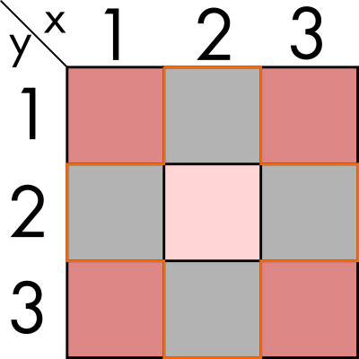
Let's imagine we have a two dimensional space, of finite size and we can discretizate it. In this first part of the exercise, for the sake of simplicity, we are going to imagine we have two dimensions: x and y with three elements each. This means we can represent it with a 3x3 array. we can also have some value for each par of coordinates, for example inhabitants in those regions. We could graphically represent it in the following way:

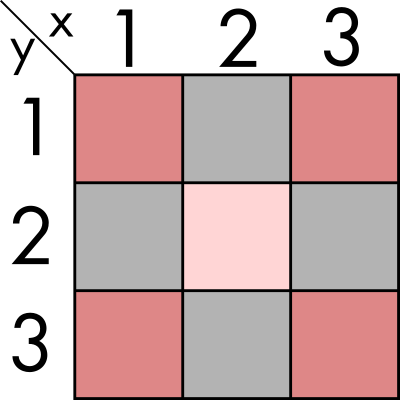
We now want to perform some statistics on the immediate neighbours, for example summing all the population around (2, 2). In this simple example, and if we also extend the neighbour condition to the diagonals, would mean aggregating all the regions in the image above. That means summing to its value, the populations of (1,1), (1,2), (1,3), (2,1), (2,3), (3,1), (3,2) and (3,3).

In this toy example we can easily identify and sum the neighbours, but I would like us to think about how to do it in a more generic and programmatic way that does not depend on us knowing the exact numbers.

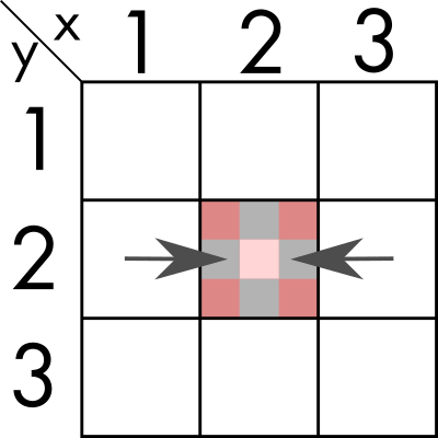
As extra limitation, we need to do it in a way that we cannot aggregate two diagonal neighbours, so we are limited only to operations in a single dimension at a time.

We can find an algorithm where we first sum over one dimension (`y` in the example). And store the resulting value in what would now be a 1-dimensional vector.

And then, we sum the values in the remaining dimension, obtaining the number for (2, 2).

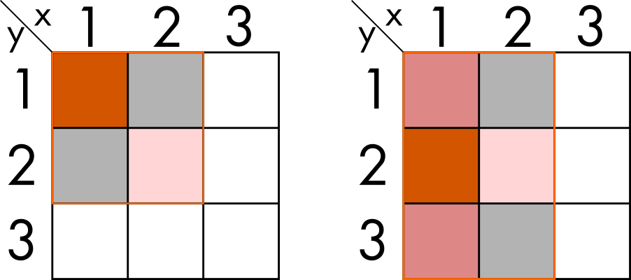
For this algorighm we need to ensure that it does not fail for the edge cases where there are not 8 neighbours, for example (1,1) that has only three, or (1,2) that has 5.

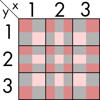
Now, if we do it for all of the regions at the same time, the result would look something like this.

Let's get out of the theory

While computing directly with matrices might be the mathematically correct way of computing this, in the real world you usually have tables, and the tables and files optimized for other statistics, and you end up with having multiple dimensions and values stored in different columns. Our example, would look like this:

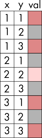
This representation is something most data engineers are used to, and plays well with how IT systems and relational databases are designed. The processing is usually done in either aggregating columns on the same row, or grouping the values and reducing the dimensionality.

In our problem however, although we might want to sum the populations we need to keep with the same number of rows, and thus being something a bit less common to do. We want to obtain Figure 5 and not Figure 3.

Luckily, the SQL operation WINDOW exists and I'm going to show to you how to use it in Spark. Let's learn how to use this operation in one dimension:

import org.apache.spark.sql.expressions.Window

val dim1Window = Window.partitionBy("y").orderBy("x").rangeBetween(-1, 1)

df.withColumn("resultDim1", sum("val") over dim1Window)

We are partitioning by the dimension we want to sum over (see example in Figure 2 and then, we order the other dimension to select only the two neighbours. We use order with rangeBetween to take into account the numerical value of x and sum only the correct neighbours.

Now, with this code, we can sum over the two dimensions:

import org.apache.spark.sql.functions.sum
import org.apache.spark.sql.{Column, DataFrame, SparkSession}

val spark = SparkSession.builder.appName("Grid").master("local[*]").getOrCreate()
import spark.implicits._

val test = (for {
  i <- 1 to 3
  j <- 1 to 3
} yield (i, j, 1)).toDF("x", "y", "val")

def sumNeighbours(df: DataFrame, targetColName: String,
                  dim1: Column, dim2: Column, sumCol: Column): DataFrame = {
  import org.apache.spark.sql.expressions.Window

  val dim1Window = Window.partitionBy(dim1).orderBy(dim2).rangeBetween(-1, 1)
  val dim2Window = Window.partitionBy(dim2).orderBy(dim1).rangeBetween(-1, 1)

  val tmpCol: String = "sum_dim1_tmp"
  val res = df.
    withColumn(tmpCol, sum(sumCol) over dim1Window).
    withColumn(targetColName, sum(tmpCol) over dim2Window)
    res.drop(tmpCol)
}


val res = sumNeighbours(test, "sum_total", $"x", $"y", $"val")
res.orderBy("x","y").show(100)
+---+---+---+---------+
|  x|  y|val|sum_total|
+---+---+---+---------+
|  1|  1|  1|        4|
|  1|  2|  1|        6|
|  1|  3|  1|        4|
|  2|  1|  1|        6|
|  2|  2|  1|        9|
|  2|  3|  1|        6|
|  3|  1|  1|        4|
|  3|  2|  1|        6|
|  3|  3|  1|        4|
+---+---+---+---------+

All in all, we have learnt that WINDOW operations are useful when we want to perform aggregations while maintaining the number of rows. Keep in mind that it can get computationally expensive and you must be careful when implementing it.

Other points of view

I've found some resources that can explain the problem (or a similar one) in a different way and might help you.

rangeBetween vs. rowsBetween

Let's try to change the method to rowsBetween. In this one, it selects the rows based on the position of it within the partition, instead of the value.

To see the effect, we must expand the example, adding some elements only some of which are populated.

In this case, the result for (1, 5) and (5,5) should be only themselves, because all their direct neighbours are empty. And if we apply the previous function, we see it gives the correct result.

val test2 = ((for {
  i <- 1 to 3
  j <- 1 to 3
} yield (i, j, 1)).toList ++ List((1, 5, 1), (5, 5, 1))).toDF("x", "y", "val")

val res2 = sumNeighbours(test2, "sum_total", $"x", $"y", $"val")
res2.orderBy("x","y").show(100)
+---+---+---+---------+
|  x|  y|val|sum_total|
+---+---+---+---------+
...
|  1|  3|  1|        4|
|  1|  5|  1|        1|
...
|  3|  3|  1|        4|
|  5|  5|  1|        1|
+---+---+---+---------+

However, when we change the method to rowsBetween method, the results no longer are the ones we expect. And it does not only affect those rows but also other ones

def sumNeighboursByRow(df: DataFrame, targetColName: String,
                  dim1: Column, dim2: Column, sumCol: Column): DataFrame = {
  import org.apache.spark.sql.expressions.Window

  val dim1Window = Window.partitionBy(dim1).orderBy(dim2).rowsBetween(-1, 1)
  val dim2Window = Window.partitionBy(dim2).orderBy(dim1).rowsBetween(-1, 1)

  val tmpCol: String = "sum_dim1_tmp"
  val res = df.
    withColumn(tmpCol, sum(sumCol) over dim1Window).
    withColumn(targetColName, sum(tmpCol) over dim2Window)
  res.drop(tmpCol)
}

val res3 = sumNeighboursByRow(test2, "sum_total", $"x", $"y", $"val")
// We will see incorrect values for (1,5) and (5,5)
// But also for (1,3) and (2,3)
res3.orderBy("x","y").show(100)
+---+---+---+---------+
|  x|  y|val|sum_total|
+---+---+---+---------+
...
|  1|  3|  1|        5|
|  1|  5|  1|        3|
...
|  2|  3|  1|        7|
...
|  5|  5|  1|        3|
+---+---+---+---------+

As a summary, you should be very cautious when to use one vs the other. If the value of the dimension ordered by is important, you should use always rangeBetween. And as bonus recommendation: always test your functions with edge cases because you might have implemented it wrong.